Evaluating Players
It can be difficult to evaluate players across basketball history. The numbers that players put up are heavily affected by the season that they are in. Pace of play, coaching style, rule changes have changed throughout the many eras of basketball. This makes it very hard to evaluate players' performance when the standards aren't uniform. Taking all of these factors into account, a player's performance can be evaluated by comparing their stats to the average. For example, Player A in Season A can average more points than Player B in Season B but Player B can still be a statistically better scorer than Player A if the average ppg was lower in Season B than in Season A.
The Z-Score
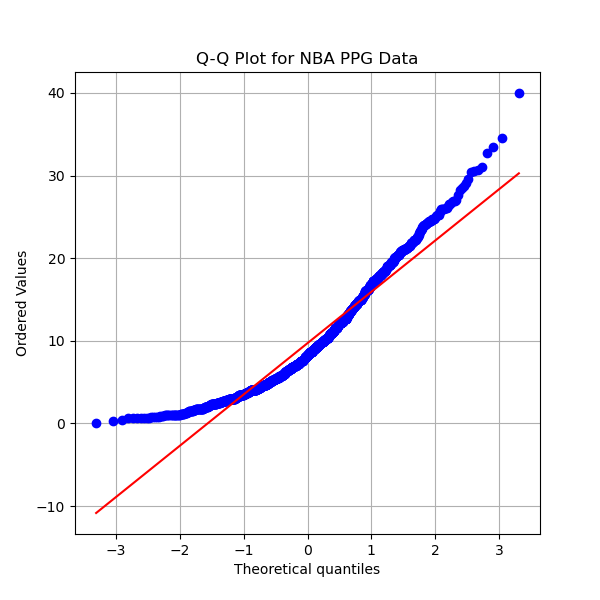
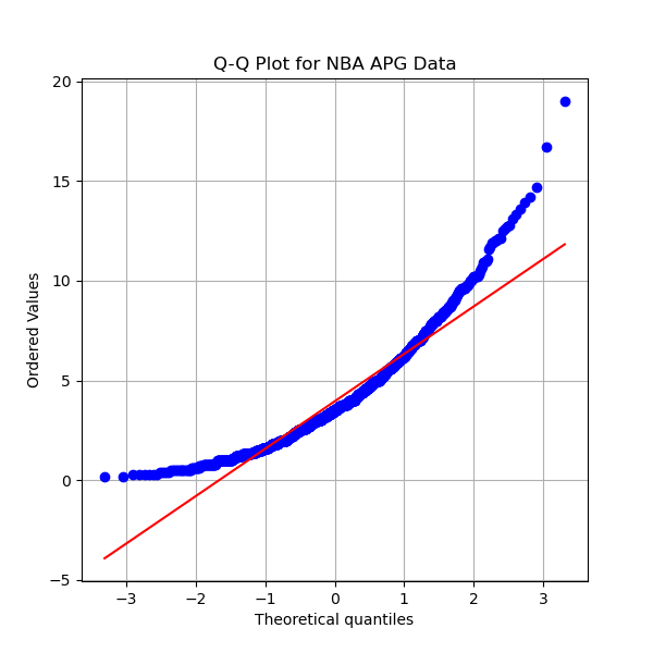
We can use the z-score of players' stats in order to evaluate players. The z-score is a statistic that uses the mean and variance in order to determine the significance of a statistic. The formula for z-score is z=x-µ/(σ^2) where x is the sample mean (player's per game average), µ is the population mean (league average per game average), and σ^2 is the variance. It is possible to test whether a sample is statistically significantly better or worse than the mean by using the z-score. The z-score only has meaning if the data follows a normal distribution, a symmetrical bell curve centered on the mean. One way to determine if data follows a normal distribution is by using a Q-Q plot. The Q-Q plots for ppg, apg, and rpg are shown below. If the scatter plot follows the red line we can assume that the data is normally distributed. The plots below show that neither ppg, apg, nor rpg are normal.

Normal Transformation
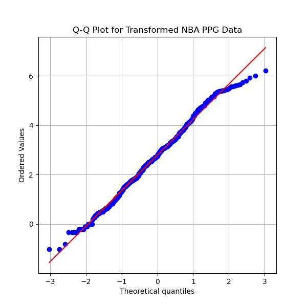
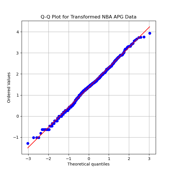
In order to use the z-score this data must be transformed into a normal distribution. The Box-Cox transformation is a method to transform data to be more normally distribution. The Box-Cox transformation is based on a parameter, λ. We can use this method in order to transform ppg, apg, and rpg into a normal distribution. After using this method on leaguewide ppg, apg, and rpg distributions the Q-Q plot looks much more normal. The plots below show that the scatter plot follows the red line relatively well. Comparing the plots above to the plots below shows the effect of the transformation. It is still an imperfect fit but some outliers are to be expected. These outliers are especially noticeable in the ppg plot, as star players tend to focus on scoring more than assisting or rebounding.

Proportions
Shooting percentages have a different formula for the z-score. Shooting percentages follow a binomial distribution. This kind of distribution can be approximated as a normal distribution if there are at least 10 successes and at least 10 fails (n*p>10 & n*(1-p)>10). The z score formula for proportions is (p̂-p)/√((p)(1-p)/n) where p̂ is the sample proportion (player's shooting percentage), p is the population proportion (league wide shooting percentage), and n is the sample size (player's shot attempts). Since increasing shot attempts minimizes the denominator, players who take more shot attempts tend to have more extreme z-scores. This means that Player A can shoot slightly worse than Player B but have a higher z-score if Player A is taking more shots. This means the z-score measures not only the ability to make shots, but also the ability to generate shots.
Significance Testing
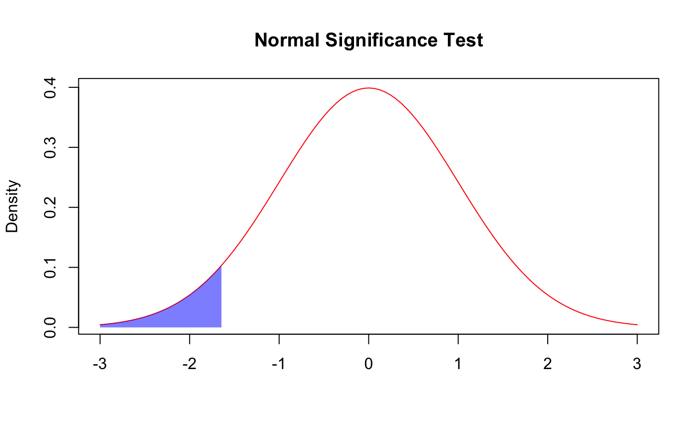
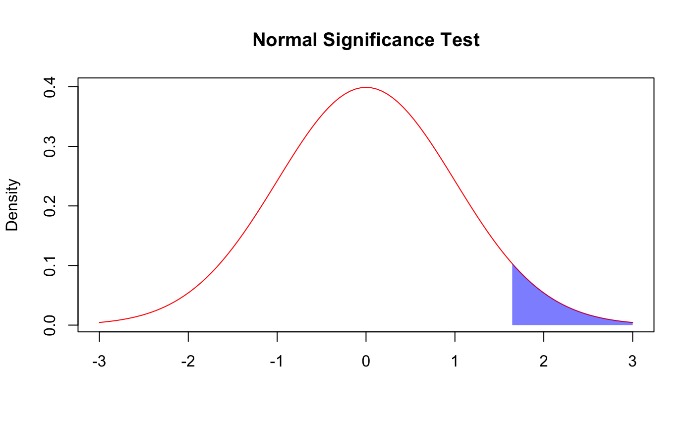
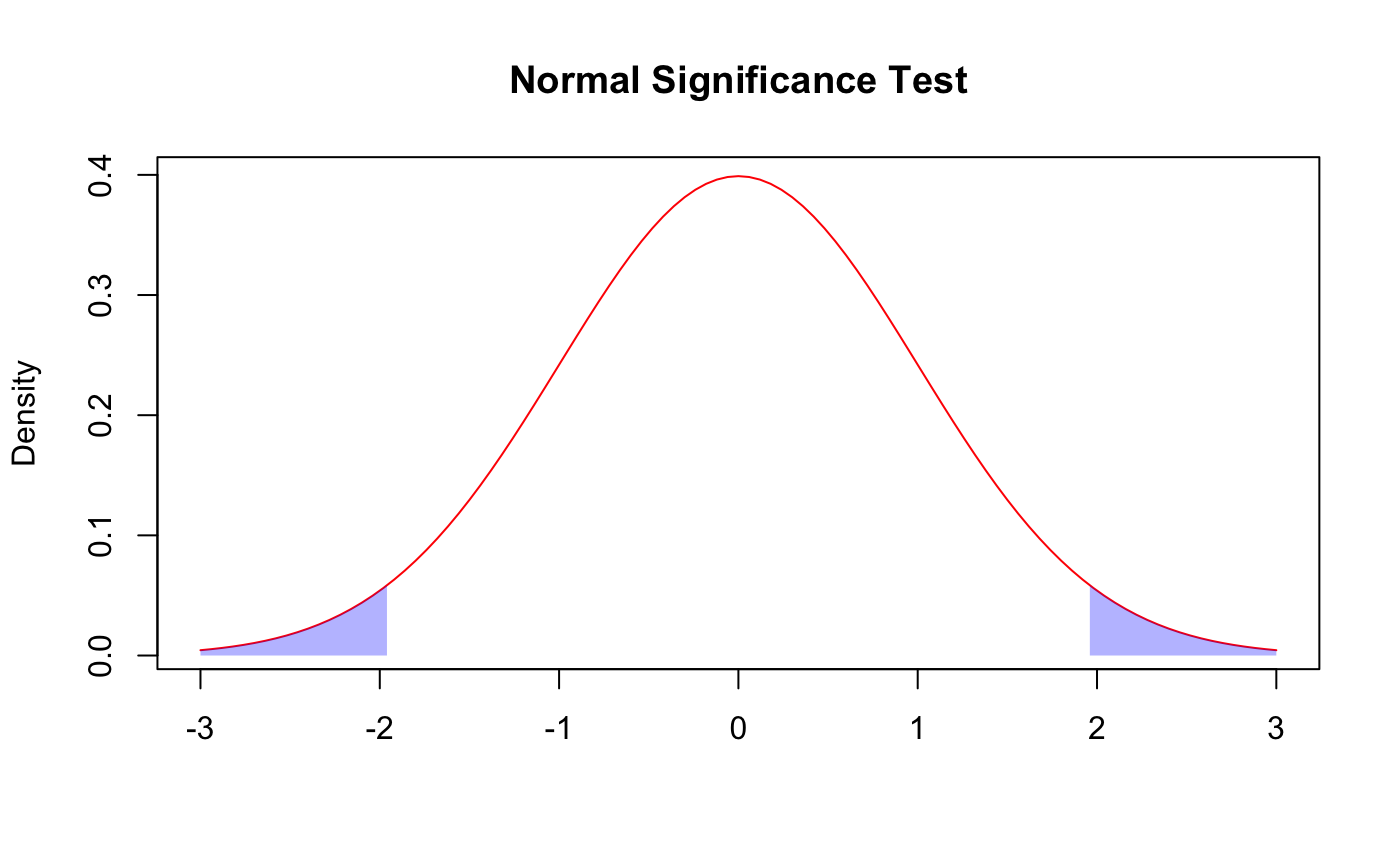
After getting the z-scores for each of the statistics, this score can be used to evaluate the performance. Since the data follows a normal distribution it can be evaluated using a significance test. Using the z-score it is possible to test the hypotheses H0:x=µ and H1:x≠µ where x is the sample mean/proportion and µ is the true population mean/proportion. Using a z-score and a normal distribution z-score table it is possible to get the probability that the sample mean would be as far from the true mean as it is given that they are equal. A significance test uses this probability, the p-value, in order to teset the 2 hypotheses above. If the p-value is below the significance level then we reject H0 and conclude that there is statistically significant evidence that the sample isn't average, if the p-value is above the significance level then we fail to reject H0, and we can't conclude that there is statistically significant evidence that the sample isn't average. For example: With a significance level of 0.05 a z-score above 1.96 has a p-value below 0.05 and we have enough evidence to conclude that this sample isn't average.
For the purposes of evaluating NBA players we either test H1:x>µ or H1:x<µ in order to determine if a player is above/below average. If the sample mean is above the population mean we test H1:x>µ and if it is below we test H1:x<µ. We can conclude that a player is well above/below average if the test finds a significant difference from the average with a significance level of 0.05. We can conclude that a player is slightly above/below average if the test finds a significant difference from the average with a significance level of 0.10 but not with a significance level of 0.05. If the test finds there is no statistically significant difference with a significance level of 0.10 then we can conclude that a player is average.